Rotors: A practical introduction for 3D graphics

When putting 3D graphics on a screen, we need a way to express rotations of the geometry we’re rendering. To avoid the problems that come with storing rotations as axes & angles, we could use quaternions. However quaternions require that we think in 4 distinct spatial dimensions, something humans are notoriously bad at. Thankfully there is an alternative that some argue is far more elegant and simpler to understand: Rotors.

Rotors come from an area of mathematics called geometric algebra. Over the past few years I’ve seen a steady increase in the number of people claiming we should bin quaternions entirely in 3D graphics and replace them with rotors. I know nothing about either so I figured I’d try out rotors. I struggled to find educational materials online that clicked well with how I think about these things though, so this post is my own explanation of rotors and the surrounding mathematical concepts. It’s written with the specific intention of implementing rotation for 3D graphics and is intended to be used partly as an educational text and partly as a reference page.

There are two sections: The first half is purely theoretical, where we’ll look at where rotors “come from”, investigate how they behave and see how we can use them to perform rotations. The second half will cover practical applications and includes example code for use-cases you’re likely to encounter in 3D graphics.

A word on notation

\(\global\def\v#1{\mathbf{#1}}\)

In this post we will write vectors, bivectors and trivectors in bold and lower-case (e.g \(\v{v}\) is a vector). Rotors will be written in bold and upper-case (e.g \(\v{R}\) is a rotor).

The basis elements of our 3D space are denoted \(\v{e_1, e_2, e_3}\), so for example \(\v{v} = v_1\v{e_1} + v_2\v{e_2} + v_3\v{e_3}\).

Where multiplication tables are given, the first argument is the entry on the far left column of the table and the second argument is the entry on the top row of the table.

Since this post is primarily concerned with 3D graphics & simulation, we will restrict our examples to 3 dimensions of space. Rotors (unlike quaternions) can easily be extended to higher dimensions but this is left as an exercise for the reader.

Theory: Adding rotors to our mathematical toolbox

Introducing: The wedge product

We begin our journey by defining a new way to combine two vectors: the so-called “wedge product”, written as \(\v{a \wedge b}\). We define the wedge product of two vectors as an associative product that distributes over addition and which is zero when both arguments are the same:

\[\begin{equation} \v{v \wedge v} = 0 \tag{ 1 } \end{equation} \]

From this we can show that the wedge product is also anticommutative:

We have yet to specify how to actually “compute” a wedge product though. We know that it produces zero when both arguments are equivalent but what if they aren’t? In this case we “compute” the wedge product by expressing the arguments in terms of its basis elements and multiplying out.

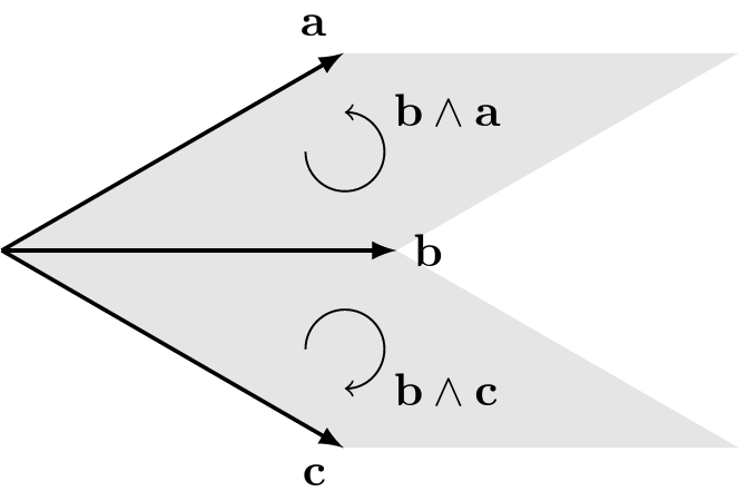
When it comes down to a pair of basis vectors we just leave them be. So for example we don’t simplify \(\v{e_1} \wedge \v{e_2}\) any further. This is because \(\v{e_1} \wedge \v{e_2}\) is not a vector. It’s a new kind of entity called a bivector. If you think of an ordinary a vector as a point (offset from the origin), then the bivector produced by applying the wedge product to those two vectors can be visualised as the infinite plane containing the origin and those two points. Equivalently, you can think of a bivector as the direction that is normal to the plane formed by the two vectors that we wedged together. The bivector \(\v{e_1 \wedge e_2}\) is in some sense the normal going in the same direction as the vector \(\v{e_3}\).

In the same way that we have basis vectors (\(\v{e_1}, \v{e_2}, \v{e_3})\), we also have basis bivectors: \(\v{e_{12}}, \v{e_{23}}, \v{e_{31}}\). Conveniently, these bivector basis elements are simple wedge products of the vector basis elements: \[ \v{e_{12}} = \v{e_1} \wedge \v{e_2} \\ \v{e_{23}} = \v{e_2} \wedge \v{e_3} \\ \v{e_{31}} = \v{e_3} \wedge \v{e_1} \]

Note that (as with vectors) we’re not restricted to a specific set of basis bivectors. Some texts prefer to use \(\v{e_{12}}, \v{e_{13}}, \v{e_{23}}\). The calculations work out a little differently but the logic is the same. For this post we’ll use \(\v{e_{12}}, \v{e_{23}}, \v{e_{31}}\) throughout. An important thing to note is that the 3-dimensional case is a little misleading here. It is very easy to confuse vectors with bivectors because they have the same number of basis elements. This is not true in higher dimensions. In 4-dimensional space, for example, there are 4 basis vectors but 6 basis bivectors so we should always explicitly state what basis elements we’re using in our calculations.

One last realisation is that in 3D we can go one step further. On top of vectors (representing lines) and bivectors (representing planes), we also have trivectors, which represent volumes. Trivectors are as far as we can go in 3D though because the space itself is 3-dimensional, there’s no room for more dimensions! Trivectors in 3D are sometimes referred to as “pseudoscalars” since they have only 1 basis element: \(\v{e_{123}}\). Trivectors in 3D are oriented (in the sense that the coefficient of the trivector basis element can be negative) but otherwise contain no positional information.

Below is a multiplication table for the wedge product of our 3D basis vectors:

\[\begin{array}{c|c:c:c} \wedge & \v{e_1} & \v{e_2} & \v{e_3} \\ \hline \v{e_1} & 0 & \v{e_{12}} & -\v{e_{31}} \\ \v{e_2} & -\v{e_{12}} & 0 & \v{e_{23}} \\ \v{e_3} & \v{e_{31}} & -\v{e_{23}} & 0 \\ \end{array}\]

Wedge product of non-basis vectors

Let us see what happens if we wedge together two arbitrary 3D vectors in the above manner:

Well now, those coefficients look awfully familiar don’t they? They’re exactly the coefficients of the usual 3D cross-product.¹ This lines up with our earlier claim that bivectors function as normals: If you look at which coefficients go with which bivector basis elements, you’ll see that the coefficient for \(\v{e_{23}}\) is the same as the coefficient of \(\v{x}\) in the usual 3D cross-product.

By virtue of “sharing” the equation for 3D vector cross product, we can conclude that the magnitude of the bivector \(\v{v \wedge u}\) is equal to the area of the parallelogram formed by \(\v{v}\) and \(\v{u}\). A neat geometric proof of this (with diagrams) can be found on the mathematics Stack Exchange. The sign of the area indicates the winding order of the parallelogram, although which direction is positive and which is negative will depend on the handedness of your coordinate system.

Like vectors, bivectors can be written as the sum of some basis elements each multiplied by some scalar. It may not come as a surprise then that as with vectors, adding two bivectors together is simply a matter of adding each of the constituent components.

So we have vector addition and bivector addition. Can we add a vector to a bivector? Yes, but we leave them as separate terms. In the same way that we don’t try to “simplify” \(\v{e_1 + e_2}\), we also don’t try to simplify \(\v{e_1 + e_{12}}\). We just leave them as the sum of these two different entities. The resulting object is neither a vector nor a bivector, but is a more general object called a “multivector”. A multivector is just a sum of scalars, vectors, bivectors, trivectors etc. All scalars, vectors, bivectors etc are also multivectors, except that they only have non-zero coefficients on one “type” of basis element. So for example you could write the vector \(\v{e_1}\) as the multivector \(\v{e_1} + 0\v{e_{12}}\).

Multivectors are particularly relevant to the discussion of our second new operation and the protagonist of this post:

Geometric product

The geometric product is defined for arbitrary multivectors, is associative, and distributes over addition. Somewhat annoyingly (in an environment involving several types of products), it is denoted with no symbol, as just \(\v{ab}\). If we have two vectors \(\v{a}\) and \(\v{b}\), we can calculate their geometric product as:

\[\begin{equation} \v{ab = (a \cdot b) + (a \wedge b)} \tag{ 2 } \end{equation} \]

Where \(\cdot\) is the usual dot product we know from traditional linear algebra. Note that if both inputs are the same then by equation 1 we get:

\[\begin{equation} \v{aa} = \v{a \cdot a} \tag{ 3 } \end{equation} \]

This, and the fact that our basis vectors are all unit-length and perpendicular to one another leads us to: \(\v{e_ie_i} = \v{e_i} \cdot \v{e_i} = 1\) and \(\v{e_ie_j} = 0 + \v{e_i} \wedge \v{e_j} = -\v{e_je_i} ~~~\forall i \neq j\).

In particular this means that \(\v{e_1e_2} = \v{e_1 \wedge e_2} = \v{e_{12}}\) (and similarly for the other basis bivectors). Indeed basis bivectors being the wedge product of basis vectors is now revealed to be a special case of being the geometric product of basis vectors. This leads us to an analogous definition for trivectors: \(\v{e_{123}} = \v{e_1e_2e_3}\).

At this point we can compute a complete multiplication table for the geometric product with basis elements in 3D:

\[\begin{array}{c|c:c:c:c:c:c:c:c} \cdot\wedge & \v{e_1} & \v{e_2} & \v{e_3} & \v{e_{12}} & \v{e_{31}} & \v{e_{23}} & \v{e_{123}} \\ \hline \v{e_1} & 1 & \v{e_{12}} & -\v{e_{31}} & \v{e_2} & -\v{e_3} & \v{e_{123}} & \v{e_{23}} \\ \v{e_2} & -\v{e_{12}} & 1 & \v{e_{23}} & -\v{e_1} & \v{e_{123}} & \v{e_3} & \v{e_{31}} \\ \v{e_3} & \v{e_{31}} & -\v{e_{23}} & 1 & \v{e_{123}} & \v{e_1} & -\v{e_2} & \v{e_{12}} \\ \v{e_{12}} & -\v{e_2} & \v{e_1} & \v{e_{123}} & -1 & \v{e_{23}} & -\v{e_{31}} & -\v{e_3} \\ \v{e_{31}} & \v{e_3} & \v{e_{123}} & -\v{e_1} & -\v{e_{23}} & -1 & \v{e_{12}} & -\v{e_2} \\ \v{e_{23}} & \v{e_{123}} & -\v{e_3} & \v{e_2} & \v{e_{31}} & -\v{e_{12}} & -1 & -\v{e_1} \\ \v{e_{123}} & \v{e_{23}} & \v{e_{31}} & \v{e_{12}} & -\v{e_3} & -\v{e_2} & -\v{e_1} & -1 \\ \end{array}\]

To compute the geometric product of two arbitrary multivectors, we can break the arguments down into their constituent basis elements and manipulate only those (using the multiplication table above). We need to do this because equations 2 and 3 above apply only to vectors, and do not apply to bivectors (or trivectors etc).

Inverses under the geometric product

Under the geometric product all non-zero vectors \(\v{v}\) have an inverse:

\[\begin{equation} \v{v}^{-1} = \frac{\v{v}}{|\v{v}|^2} \tag{ 4 } \end{equation} \]

Similarly, the geometric product of two vectors \(\v{a}\) and \(\v{b}\) also has an inverse:

\[\begin{equation} (\v{ab})^{-1} = \v{b}^{-1}\v{a}^{-1} \tag{ 5 } \end{equation} \]

Since every vector has an inverse, for any two vectors \(\v{a}\) and \(\v{b}\) we can write: \[\begin{aligned} \v{a} &= \v{a} \\ \v{a} &= \v{abb}^{-1} \\ \v{a} &= \frac{1}{|\v{b}|^2} \v{(ab)b} \\ \v{a} &= \frac{1}{|\v{b}|^2} \v{(a \cdot b + a \wedge b) b} \\ \v{a} &= \frac{\v{a \cdot b}}{|\v{b}|^2} \v{b} + \frac{\v{a \wedge b}}{|\v{b}|^2} \v{b} \\ \end{aligned}\]

From this we conclude that for two arbitrary (non-zero) vectors \(\v{a}\) and \(\v{b}\), we can write one in terms of components parallel and perpendicular to the other:

\[\begin{equation} \v{a} = \v{a}_{\parallel b} + \v{a}_{\perp b} \tag{ 6 } \end{equation} \]

Where \(\v{a_{\parallel b}}\) is the component of \(\v{a}\) parallel to \(\v{b}\) (the projection of \(\v{a}\) onto \(\v{b}\)) and \(\v{a_{\perp b}}\) is the component of \(\v{a}\) perpendicular to \(\v{b}\) (the rejection of \(\v{a}\) from \(\v{b}\)). We know from linear algebra that

\[\begin{equation} \v{a_{\parallel b}} = \frac{\v{a \cdot b}}{|\v{b}|^2}\v{b} \tag{ 7 } \end{equation} \]

Substituting into the calculation above we get \(\v{a} = \v{a_{\parallel b}} + \frac{\v{a \wedge b}}{|\v{b}|^2} \v{b} \) from which we conclude that

\[\begin{equation} \v{a_{\perp b}} = \frac{\v{a \wedge b}}{|\v{b}|^2}\v{b} \tag{ 8 } \end{equation} \]

Reflections with the geometric product

Recall from linear algebra that given two non-zero vectors \(\v{a}\) and \(\v{v}\), we can write the reflection of \(\v{a}\) over \(\v{v}\) as:

\[ \v{a^\prime} = \v{a} - 2\v{a_{\perp v}} = \v{a}_{\parallel v} - \v{a}_{\perp v} \]

If we substitute equations 7 and 8 we get:

\[\begin{aligned} \v{a^\prime} &= \v{a}_{\parallel v} - \v{a}_{\perp v} \\ &= \frac{\v{v \cdot a}}{|\v{a}|^2} \v{a} - \frac{\v{v \wedge a}}{|\v{a}|^2} \v{a} \\ &= (\v{v \cdot a})\frac{\v{a}}{|\v{a}|^2} - (\v{v \wedge a})\frac{\v{a}}{|\v{a}|^2} \\ &= \v{(v \cdot a)a}^{-1} - (\v{v \wedge a})\v{a}^{-1} \\ &= \v{(a \cdot v)a}^{-1} + (\v{a \wedge v})\v{a}^{-1} \\ &= (\v{a \cdot v + a \wedge v})\v{a}^{-1} \\ &= \v{(av)a}^{-1} \\ \v{a^\prime} &= \v{ava}^{-1} \\ \end{aligned}\]

So we can reflect vectors using only the geometric product. \(\v{ava}^{-1}\) is a form we will see quite often, and is sometimes referred to as a “sandwich product”.

The first and last lines of the calculation above together demonstrate an important property: Since \(\v{ava}^{-1} = \v{a}_{\parallel v} - \v{a}_{\perp v}\), we know that \(\v{ava}^{-1}\) is just a vector and contains no scalar, bivector (or trivector etc) components. This means we can use the output of such a sandwich product as the input to another sandwich product, which we will do shortly.

For our own convenience, we can also produce an equation for the output of such a sandwich product:

Rotors as a combination of two reflections

Now that we can safely achieve reflection of one vector over another by way of a geometric sandwich product, rotations are right around the corner: We just reflect twice.

Let \(\v{v}\) be our input vector (the one we’d like to rotate) and say we’d like to reflect over the vectors \(\v{a}\) and then \(\v{b}\). This is just a pair of sandwich products: \(\v{v}^{\prime\prime} = \v{bv}^\prime\v{b}^{-1} = \v{bava}^{-1}\v{b}^{-1}\). If we let \(\v{R = ba}\) then by equation 5 this can be conveniently written as: \(\v{v}^{\prime\prime} = \v{RvR}^{-1}\) and \(\v{R}\) is our rotor.

To see how this works, consider the following example and corresponding diagrams:

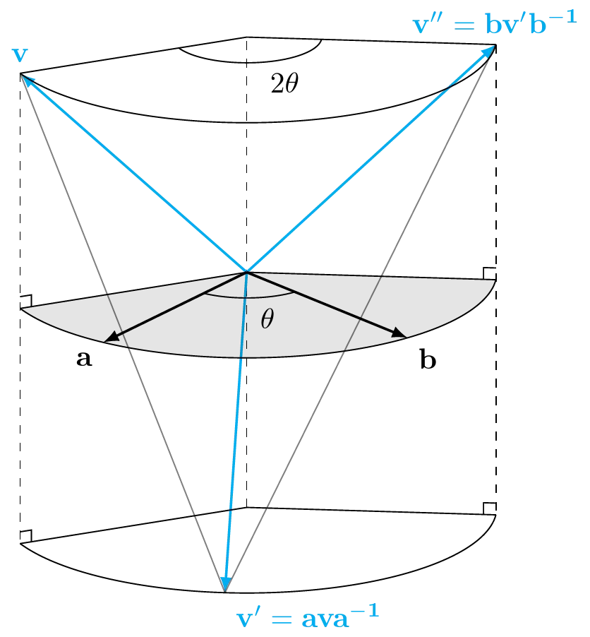
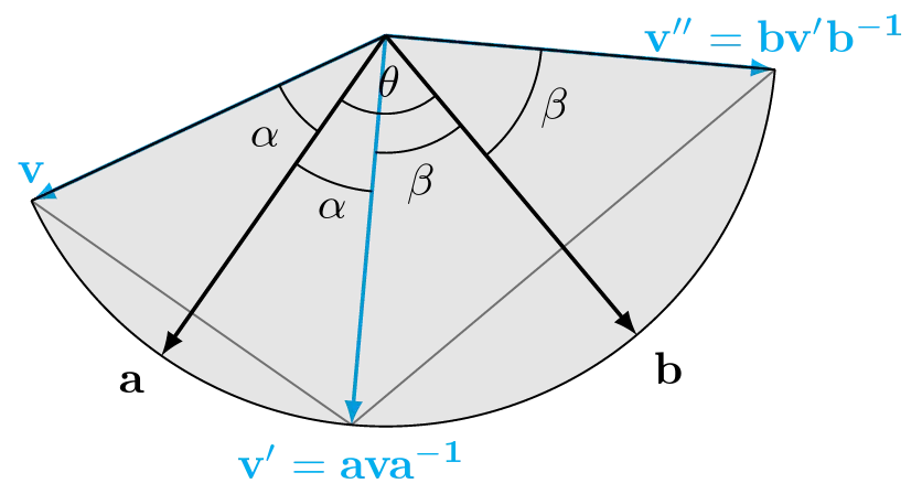
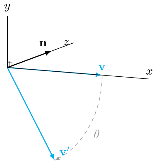
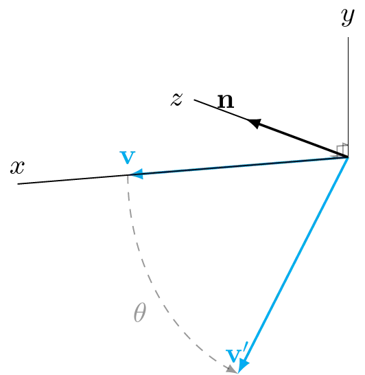
You can see in the 2D diagram on the right, how each reflection inverts the angle between the input vector and the vector it’s being reflected across. In doing so twice, we have produced a total rotation by twice the angle between the two reflection vectors.

If you were to look only at the 2D diagram on the right however, you might be thinking that we only needed a single reflection. You could indeed get from one point on the circle to any other point on the circle by reflecting over just one appropriately selected vector but this wouldn’t actually be a rotation. The 3D diagram on the left demonstrates one of the reasons why this is not sufficient: We’d end up on the wrong side of the plane of reflection. Having two reflections allows us to “rotate” part of the way with the first reflection, flipping over to the other side of the plane of rotation, and the second rotation “rotates” us the rest of the way around while getting us back across the plane of rotation to our intended rotated vector.

Does that mean that a single vector would be sufficient in 2D? Well no we still need two, because there’s another problem: Reflection is simply not the same transformation as rotation and will, well…reflect…the relative positions of the vectors it’s applied to. Here’s the same example, but with two extra initial vectors, offset slightly from \(\v{v}\):

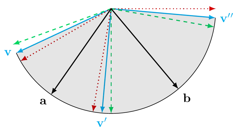
You can see how our 3 input vectors are in the wrong “order” (if you imagine going around the circle) after the first reflection, but that is fixed by the second reflection.

I confess that this is a slightly hand-wavey geometric justification that leans on one’s intuition for what reflections and rotations should look like. For the stout of heart, Jaap Suter provides a more rigorous algebraic derivation.

The identity rotor

When using rotors for rotation, you are likely to very quickly run into a situation where you want a “no-op” rotation. A rotation which transforms any input vector into itself. You want an identity rotor.

Any rotor that contains only a scalar component is an identity rotor. To see this, recall that we constructed our rotors as the geometric product of two vectors (\(\v{R} = \v{ba}\)). The rotor \(\v{R}\) produces a rotation by twice the angle between \(\v{a}\) and \(\v{b}\). If that angle is zero then twice that angle is still zero and the rotor will produce no rotation. If the angle between the two vectors is zero then we can express one of those vectors as a scalar multiple of the other (\(\v{b} = s\v{a}\) for \(\v{s \in \mathbb{R}}\)). Applying equation 2 then gives \[\begin{aligned} \v{R} &= \v{b \cdot a + b \wedge a} \\ &=(s\v{a}) \cdot \v{a} + (s\v{a}) \wedge \v{a} \\ &=s(\v{a} \cdot \v{a}) + s(\v{a} \wedge \v{a}) \\ &=s|a|^2 + s(0) \\ &=s|a|^2 \end{aligned}\]

Since we’ve placed no restrictions on \(s\) or \(\v{a}\), we may choose \(\v{a} = (1, 0, 0) \implies |a| = 1 \implies \v{R} = 1\).

Axis-angle representation for rotors

Recall from regular vector algebra that \(\v{a \cdot b} = |a| |b| cos\theta\) and \(|\v{a \times b}| = |\v{a \wedge b}| = |a| |b| sin\theta\). With this we can modify equation 2 to get an “axis-angle-like” representation:

\[\begin{aligned} \v{R} &= \v{ba} \\ &= \v{b \cdot a + b \wedge a} \\ &= \v{b \cdot a} + |b \wedge a| \left(\frac{\v{b \wedge a}}{|b \wedge a|}\right) \\ &= |b||a|cos\theta + |b||a|sin\theta \left(\frac{\v{b \wedge a}}{|b \wedge a|}\right) \\ \end{aligned}\]

If we consider just the case where \(\v{a}\) and \(\v{b}\) are unit vectors separated by an angle \(\theta\) then \(|b||a| = 1\) and we can change variables to \(\v{n} = \frac{\v{b \wedge a}}{|b \wedge a|}\) the unit bivector “plane” spanning \(\v{a}\) and \(\v{b}\), to get:

\[ \v{R} = cos\theta + sin\theta \v{n} \]

Finally, recall that the rotor will produce a rotation equal to twice the angle between its constituent vectors and so we should actually use only half of the input angle:

\[\begin{equation} \v{R} = cos\left(\frac{\theta}{2}\right) + sin\left(\frac{\theta}{2}\right) \v{n} \tag{ 13 } \end{equation} \]

Which direction this rotation goes in (clockwise or counter-clockwise) depends on the handedness of your coordinate system, as seen in the example below:

If you want to claim that a rotation is clockwise or counter-clockwise you need to give a reference viewpoint. If your reference is “looking along the axis” then the rotation in left-handed coordinates is going clockwise, while in the right-handed coordinates it’s counter-clockwise.

Applications: Putting rotors to work

Now that we’ve seen the theory of rotors, let’s turn our attention to more practical concerns. Below is a small collections of answers to questions I encountered myself when implementing rotors, with C++ code for reference.

How do I store a rotor in memory?

A rotor is just the geometric product of the two vectors that form the plane of rotation. In 3D it contains a scalar component and 3 bivector components. So we just store it as a tuple of 4 numbers (as we would a 4D vector used in the usual homogeneous coordinates setup)

struct rotor3
{
    float scalar;
    float xy;
    float yz;
    float zx;
};

How do I represent an orientation (as opposed to a rotation)?

Rotors (like quaternions) encode rotations. Transforms that, when applied to an orientation, produce a new orientation. There is no such thing as “a rotor pointing along the X-axis”, for example. This is great when we have something with a particular orientation (e.g a player character facing down the X axis) and want to transform it to some other orientation (e.g you want your player character to instead face down the Z axis), but doesn’t immediately help us encode “the player character is facing down the X axis” in the first place.

Thankfully we can select a convention for a “default” orientation (“facing down the X axis” for example) and then encode all orientations as rotations away from that default orientation.

How do I produce a rotor representing a rotation from orientation A to orientation B?

Let’s represent an orientation as a unit vector along the “forward” direction of the orientation. Now we have two vectors representing the initial and final orientations and we want to rotate from the initial vector to the final vector.

We could create a rotor just from those two vectors directly, but while that would produce a rotation in the correct plane in the correct direction, it would rotate twice as far as we’d like (since the rotation you get by applying a rotor to a vector is twice the angle between the two vectors that defined the rotor). The naive approach would be to compute the angle between our two vectors and then use an existing axis-angle rotation function to produce a “half-way” vector and then construct our rotor from that:

vec3 axis_angle_rotate(vec3 axis, float angle, vec3 vector_to_rotate);

rotor3 from_to_naive(vec3 from_dir, vec3 to_dir)
{
    // Calculations below assume the input directions are normalised
    from_dir = from_dir.normalized();
    to_dir = to_dir.normalized();

    // Get the angle between the input directions
    const float theta = acosf(dot(from_dir, to_dir));

    // Get the axis of rotation/normal of the plane of rotation
    const vec3 axis = cross(from_dir, to_dir).normalized();

    // Compute the second vector for our rotor, half way between from_dir and to_dir
    const vec3 halfway = axis_angle_rotate(axis, theta*0.5f, from_dir);

    const vec3 wedge = {
        (halfway.x * from_dir.y) - (halfway.y * from_dir.x),
        (halfway.y * from_dir.z) - (halfway.z * from_dir.y),
        (halfway.z * from_dir.x) - (halfway.x * from_dir.z),
    };
    rotor3 result = {};
    result.scalar = dot(from_dir, halfway);
    result.xy = wedge.x;
    result.yz = wedge.y;
    result.zx = wedge.z;
    return result;
}

Of course this assumes the existence of an axis_angle_rotate() function, but thankfully equation 13 provides exactly that. If we normalise the from- and to-vectors and denote the resulting directions as \(\v{a}\) and \(\v{b}\) respectively then we can get the angle between them as \(\theta = cos^{-1}(\v{a \cdot b})\) and our from-to rotor is:

\[\begin{equation} \v{R} = cos\left(\frac{\theta}{2}\right) + sin\left(\frac{\theta}{2}\right)\left(\frac{\v{b \wedge a}}{|b \wedge a|}\right) \tag{ 14 } \end{equation} \]

rotor3 from_to_rotor(vec3 from_dir, vec3 to_dir)
{
    // Calculations below assume the input directions are normalised
    from_dir = from_dir.normalized();
    to_dir = to_dir.normalized();

    // Get the angle between the input directions
    const float theta = acosf(dot(from_dir, to_dir));
    const float cos_half_theta = cosf(theta * 0.5f);
    const float sin_half_theta = sinf(theta * 0.5f);

    // Compute the normalized "to_dir wedge from_dir" product
    const vec3 wedge = vec3 {
        (to_dir.x * from_dir.y) - (to_dir.y * from_dir.x),
        (to_dir.y * from_dir.z) - (to_dir.z * from_dir.y),
        (to_dir.z * from_dir.x) - (to_dir.x * from_dir.z),
    }.normalized();

    rotor3 result = {};
    result.scalar = cos_half_theta;
    result.xy = sin_half_theta * wedge.x;
    result.yz = sin_half_theta * wedge.y;
    result.zx = sin_half_theta * wedge.z;
    return result;
}

This will be correct but requires us to do a bunch of trigonometry and if we could achieve the same thing without trigonometry then that might be faster (but as with all performance-motivated changes, you should measure it).

Recall that a rotor defined as the product of two vectors will produce a rotation from one toward the other. The problem is that it will produce a rotation by twice the angle between the input vectors, so it will “rotate past” our destination vector if we just used the product of our input vectors. Naturally then, we could swap out one of the arguments for a vector that is half-way between from and to such that twice the rotation will be precisely what we’re looking for!

rotor3 from_to_rotor_notrig(vec3 from_dir, vec3 to_dir)
{
    from_dir = from_dir.normalized();
    to_dir = to_dir.normalized();

    const vec3 halfway = (from_dir + to_dir).normalized();

    const vec3 wedge = {
        (halfway.x * from_dir.y) - (halfway.y * from_dir.x),
        (halfway.y * from_dir.z) - (halfway.z * from_dir.y),
        (halfway.z * from_dir.x) - (halfway.x * from_dir.z),
    };
    Rotor3 result = {};
    result.scalar = from_dir.dot(halfway);
    result.xy = wedge.x;
    result.yz = wedge.y;
    result.zx = wedge.z;
    return result;
}

I should note, however, that both of these implementations have at least one downside: They fail at (or very close to) from_dir == -to_dir. In the trigonometry-free version, this is because at that point the “halfway” vector will be zero and can’t be normalized so you’ll get garbage. You’d need to either be sure this will not happen or check for it and do something else in that case.

How do I append/combine/multiply two (or more) rotors?

Rotors can be combined by just multiplying them together with the geometric product. We know that a rotor \(\v{R}\) is applied to a vector \(\v{v}\) by way of the sandwich product \(\v{v}^\prime = \v{RvR}^{-1}\) so if we had two rotors \(\v{R}_1\) and \(\v{R}_2\) we’d just apply them in order: \(\v{v}^\prime = \v{R}_2\v{R}_1\v{v}\v{R}_1^{-1}\v{R}_2^{-1} = (\v{R}_2\v{R}_1)\v{v}(\v{R}_2\v{R}_1)^{-1}\) and we see that the combined rotor \(\v{R}_3 = \v{R}_2\v{R}_1\).

Of course this only works if the product of two rotors is again a rotor. In order to convince ourselves that this is the case we can just do the multiplication:

This multiplication also translates fairly directly into code:

rotor3 combine(rotor3 lhs, rotor3 rhs)
{
    rotor3 result = {};
    result.scalar = lhs.scalar*rhs.scalar - lhs.xy*rhs.xy - lhs.yz*rhs.yz - lhs.zx*rhs.zx;
    result.xy = lhs.scalar*rhs.xy + lhs.xy*rhs.scalar - lhs.yz*rhs.zx + lhs.zx*rhs.yz;
    result.yz = lhs.scalar*rhs.yz + lhs.xy*rhs.zx + lhs.yz*rhs.scalar - lhs.zx*rhs.xy;
    result.zx = lhs.scalar*rhs.zx - lhs.xy*rhs.yz + lhs.yz*rhs.xy + lhs.zx*rhs.scalar;
    return result;
}

How do I invert or reverse a rotor to produce the same rotation in the opposite direction?

Since the rotor produced by the geometric product of vectors \(\v{ba}\) is a rotation in the plane formed by those two vectors, by twice the angle between those vectors (in the direction from a to b), we can produce a rotation in the same plane by the same angle in the opposite direction by just swapping \(\v{a}\) and \(\v{b}\) to get: \(\v{R}^\prime = \v{ab} = \v{a \cdot b + a \wedge b} = \v{b \cdot a - b \wedge a}\) which we can produce with very little computation from \(\v{R}\) by just negating the bivector components:

rotor3 reverse(rotor3 r)
{
    rotor3 result = {};
    result.scalar = r.scalar,
    result.xy = -r.xy;
    result.yz = -r.yz;
    result.zx = -r.zx;
    return result;
}

Given a particular rotor, how do I actually apply it to a vector directly?

Earlier when we showed how to apply a rotor, we did it in two steps as two separate reflection calculations. While mathematically equivalent, this requires that we store the vectors that make up our rotor (rather than just the scalar & bivector components) and requires us to do far more arithmetic. Instead we’ll sandwich the input vector directly with the entire, pre-computed rotor:

These calculations can be fairly directly translated into code that we can apply to our rotor and vector types. Note that the code below assumes our rotor was constructed from two unit vectors (which is something we enforced in our from_to() code above).

vec3 transform(rotor3 r, vec3 v) const
{
    // Assume r is formed by the multiplication of two unit vectors.
    // Then S = Rv, result = SR^{-1} where R^{-1} is just R with the bivector coefficients negated
    const float S_x = r.scalar*v.x + r.xy*v.y - r.zx*v.z;
    const float S_y = r.scalar*v.y - r.xy*v.x + r.yz*v.z;
    const float S_z = r.scalar*v.z - r.yz*v.y + r.zx*v.x;
    const float S_xyz = r.xy*v.z + r.yz*v.x + r.zx*v.y;

    vec3 result = {};
    result.x = S_x*r.scalar +   S_y*r.xy + S_xyz*r.yz -   S_z*r.zx;
    result.y = S_y*r.scalar -   S_x*r.xy +   S_z*r.yz + S_xyz*r.zx;
    result.z = S_z*r.scalar + S_xyz*r.xy -   S_y*r.yz +   S_x*r.zx;
    return result;
}

How do I convert a rotor to a matrix so I can use it in my graphics pipeline?

Think of rotation as a change of basis. We’re changing from the standard basis (the \(x\), \(y\) and \(z\) axes) to a new basis which is just the standard basis after undergoing our rotation.

As we know from linear algebra, the matrix that applies this change of basis is simply the one whose columns are the new (rotated) basis vectors (assuming you’re using column vectors).

Conveniently, showed how to apply a rotor to a vector directly above, so we can use that to transform each of the standard basis vectors and output a matrix with those vectors as its columns (and padded with zeroes to make it 4x4):

mat4 rotate(rotor3 r)
{
    const vec3 new_x = transform(r, vec3{1.0f, 0.0f, 0.0f});
    const vec3 new_y = transform(r, vec3{0.0f, 1.0f, 0.0f});
    const vec3 new_z = transform(r, vec3{0.0f, 0.0f, 1.0f});
    
    mat4 result = {};
    result.columns[0] = vec4{new_x.x, new_x.y, new_x.z, 0.0f},
    result.columns[1] = vec4{new_y.x, new_y.y, new_y.z, 0.0f},
    result.columns[2] = vec4{new_z.x, new_z.y, new_z.z, 0.0f},
    result.columns[3] = vec4{0.0f, 0.0f, 0.0f, 1.0f},
    return result;
}

The many zeroes in our input vectors suggest that mathematically there will be many intermediate calculations that end up as zero and could be skipped. If you need extra performance you could try inlining transform() and removing all the multiplications by zero.

How do I turn a quaternion into an equivalent (3D) rotor?

Given the number of similarities between quaternions and 3D rotors, it may not come as a surprise that they are in fact effectively the same mathematical object (they’re isomorphic). All we need to turn one into the other is to know which quaternion basis elements correspond to which rotor basis elements.

By multiplying out our transform-a-vector-using-a-rotor calculations above and comparing the results to the quaternion representation of the Euler-Rodrigues formula, we get the following mappings:

\[ \v{i} \to \v{-e_{23}} \\ \v{j} \to \v{-e_{31}} \\ \v{k} \to \v{-e_{12}} \\ \]

and the scalar components stay as the scalar components. Our transformation is therefore:

struct UnitQuaternion
{
    float w; // scalar component
    float x; // coefficient of i
    float y; // coefficient of j
    float z; // coefficient of k
};

rotor3 quaternion_to_rotor3(UnitQuaternion q)
{
    rotor3 result = {};
    result.scalar = q.w;
    result.xy = -q.z;
    result.yz = -q.x;
    result.zx = -q.y;
    return result;
}

How do I smoothly & correctly interpolate between two rotors?

Rotors (in 3D) are 4D vectors. To simplify many calculations, we’ve added the requirement that they’re 4D unit vectors. While there are many ways to interpolate between two 4D unit vectors, we will cover just two of them (the two you are most likely to use).

The first and simplest way to interpolate between two rotors is just standard 4D vector lerp() with the extra step to re-normalise the resulting value, sometimes called nlerp():

float lerp(float a, float b, float t);

rotor3 nlerp_incorrect(rotor3 lhs, rotor3 rhs, float t)
{
    rotor3 r = {};
    r.scalar = lerp(lhs.scalar, rhs.scalar, t);
    r.xy = lerp(lhs.xy, rhs.xy, t);
    r.yz = lerp(lhs.yz, rhs.yz, t);
    r.zx = lerp(lhs.zx, rhs.zx, t);

    const float magnitude = sqrtf(r.scalar*r.scalar + r.xy*r.xy + r.yz*r.yz + r.zx*r.zx);
    r.scalar /= magnitude;
    r.xy /= magnitude;
    r.yz /= magnitude;
    r.zx /= magnitude;
    return r;
}

We’ll get back to the reason why this function is marked as incorrect in a minute. First let’s take a look at the other approach: slerp():

Slerp (“Spherical linear interpolation”) was introduced by Ken Shoemake in a SIGGRAPH paper in 1985 for the purpose of interpolating quaternions (which are isomorphic to rotors). Wikipedia helpfully summarises it as:

\[ \text{slerp}(\v{a}, \v{b}, t) = \frac{sin((1-t)\theta)}{sin(\theta)}\v{a} + \frac{sin(t\theta)}{sin(\theta)}\v{b} \]

where \(\theta\) is the angle between \(\v{a}\) and \(\v{b}\). This translates fairly directly into code as:

rotor3 slerp_incorrect(rotor3 from, rotor3 to, float t)
{
    // Assume that `from` and `to` both have magnitude 1
    // (IE they are the product of two unit vectors)
    // then cos(theta) = dot(from, to)
    const float cos_theta = from.scalar*to.scalar + from.xy*to.xy + from.yz*to.yz + from.zx*to.zx;

    const float theta = acosf(cos_theta);
    const float from_factor = sinf((1.0f - t)*theta)/sinf(theta);
    const float to_factor = sinf(t*theta)/sinf(theta);

    rotor3 result = {};
    result.scalar = from_factor*from.scalar + to_factor*to.scalar;
    result.xy = from_factor*from.xy + to_factor*to.xy;
    result.yz = from_factor*from.yz + to_factor*to.yz;
    result.zx = from_factor*from.zx + to_factor*to.zx;
    return result;
}

Both of these functions have been marked as “incorrect”. That is because they both suffer from the same problem: They don’t always give us the shortest path between the two inputs.

As we saw earlier, rotors lend themselves quite easily to the “axis-angle” view of rotations (equation 13). So let’s compare two axis-angle-type rotations: Picture, if you can, a rotation of 30 degrees clockwise around the positive Z axis. Now picture a rotation of 30 degrees counter-clockwise around the negative Z axis. These rotations are equivalent. Negating both the axis and the angle produces an equivalent rotation and this is exactly what happens if we negate each component of a rotor, so given a rotor \(\v{R}\), both \(\v{R}\) and \(\v{-R}\) represent the same rotation.

If we’re only using our rotor to transform vectors then this fact is irrelevant, but if we want to interpolate between to rotors then it needs to be considered. If we tried to interpolate between two rotors that where going “in the opposite direction”, our interpolation would take the long way around rather than the short way.

Thankfully controlling this is very easy: We just need to make sure that the dot product of our two rotors (taken as if they were 4D vectors) is positive.

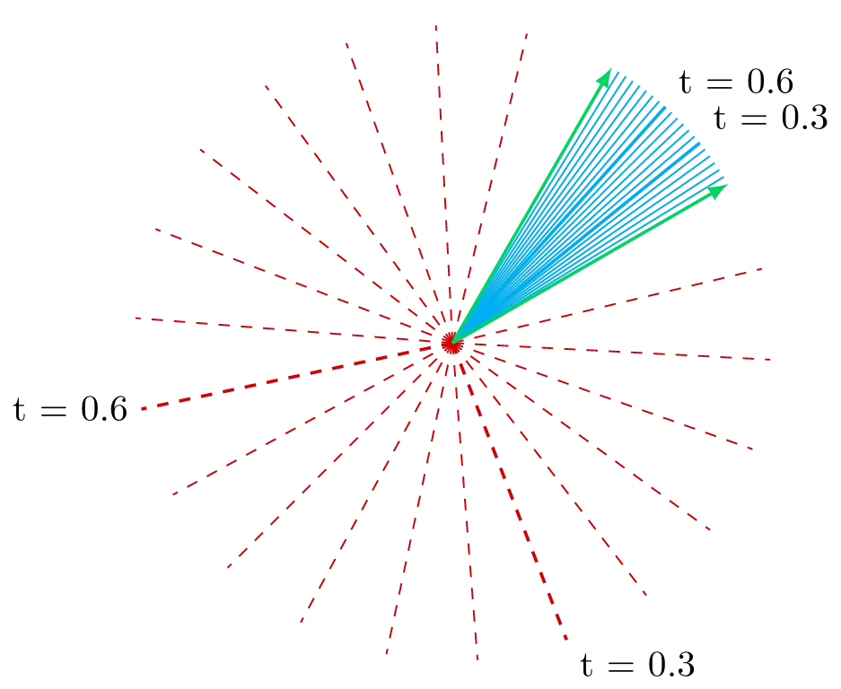
The diagram below is an illustration of this effect. Here we have two green arrows, each representing a different rotor being applied to the same input vector. The solid blue lines and the dashed red lines are the results of using slerp() to interpolate between those rotors. If the dot product between the two rotors is positive, we get the solid blue lines. If it is negative, we get the dashed red lines.

So under the assumption that we’re almost always going to want the shorter path between our input rotors, let’s amend our two functions:

rotor3 nlerp(rotor3 lhs, rotor3 rhs, float t)
{
    const float dot = from.scalar*to.scalar + from.xy*to.xy + from.yz*to.yz + from.zx*to.zx;
    if(dot < 0.0f)
    {
        to.scalar = -to.scalar;
        to.xy = -to.xy;
        to.yz = -to.yz;
        to.zx = -to.zx;
    }

    rotor3 r = {};
    r.scalar = lerp(lhs.scalar, rhs.scalar, t);
    r.xy = lerp(lhs.xy, rhs.xy, t);
    r.yz = lerp(lhs.yz, rhs.yz, t);
    r.zx = lerp(lhs.zx, rhs.zx, t);

    const float magnitude = sqrtf(r.scalar*r.scalar + r.xy*r.xy + r.yz*r.yz + r.zx*r.zx);
    r.scalar /= magnitude;
    r.xy /= magnitude;
    r.yz /= magnitude;
    r.zx /= magnitude;
    return r;
}

rotor3 slerp_stillincorrect(rotor3 from, rotor3 to, float t)
{
    float dot = from.scalar*to.scalar + from.xy*to.xy + from.yz*to.yz + from.zx*to.zx;
    if(dot < 0.0f)
    {
        to.scalar = -to.scalar;
        to.xy = -to.xy;
        to.yz = -to.yz;
        to.zx = -to.zx;
    }

    // Assume that `from` and `to` both have magnitude 1
    // (IE they are the product of two unit vectors)
    // then cos(theta) = dot(from, to)
    const float cos_theta = dot;

    const float theta = acosf(cos_theta);
    const float from_factor = sinf((1.0f - t)*theta)/sinf(theta);
    const float to_factor = sinf(t*theta)/sinf(theta);

    rotor3 result = {};
    result.scalar = from_factor*from.scalar + to_factor*to.scalar;
    result.xy = from_factor*from.xy + to_factor*to.xy;
    result.yz = from_factor*from.yz + to_factor*to.yz;
    result.zx = from_factor*from.zx + to_factor*to.zx;
    return result;
}

Unfortunately, our slerp() implementation is still incorrect. It still suffers from a numerical issue when the angle between from and to is very close (or exactly equal) to 0, causing us to divide by a value that is very close (or exactly equal) to 0. Another possibility is that because floating-point numbers on actual, real-life computers have limited precision we could find ourselves in a situation where our dot product is actually greater than 1, leaving it outside of the domain of \(cos^{-1}\).

A common workaround for all of this is to just switch to nlerp() when the input rotors are very similar (dot product is very close to \(1\)):

rotor3 slerp(rotor3 from, rotor3 to, float t)
{
    float dot = from.scalar*to.scalar + from.xy*to.xy + from.yz*to.yz + from.zx*to.zx;
    if(dot < 0.0f)
    {
        to.scalar = -to.scalar;
        to.xy = -to.xy;
        to.yz = -to.yz;
        to.zx = -to.zx;
        dot = -dot;
    }

    // Avoid numerical stability issues with trig functions when
    // the angle between `from` and `to` is close to zero.
    // Also assumes `from` and `to` both have magnitude 1.
    if(dot > 0.99995f)
    {
        return nlerp(from, to, t);
    }

    // Assume that `from` and `to` both have magnitude 1
    // (IE they are the product of two unit vectors)
    // then cos(theta) = dot(from, to)
    const float cos_theta = dot;

    const float theta = acosf(cos_theta);
    const float from_factor = sinf((1.0f - t)*theta)/sinf(theta);
    const float to_factor = sinf(t*theta)/sinf(theta);

    rotor3 result = {};
    result.scalar = from_factor*from.scalar + to_factor*to.scalar;
    result.xy = from_factor*from.xy + to_factor*to.xy;
    result.yz = from_factor*from.yz + to_factor*to.yz;
    result.zx = from_factor*from.zx + to_factor*to.zx;
    return result;
}

So now we have two complete methods for interpolating between rotors. Great. Why did we need two?

Consider using both to interpolate between two orientations:

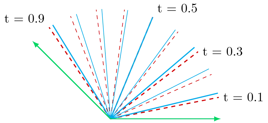
slerp() produces values that are spaced evenly apart, while nlerp() produces values that are further apart around \(t = 0.5\) and closer together around \(t = 0\) and \(t = 1\). If this were an animation and \(t\) were the elapsed time, this would show up as the animation playing slightly more quickly near the beginning and end, and slightly more slowly around the middle.

How much of a problem this is depends on your use-case. If people are going to be watching very closely and execution speed is not a concern, you probably want slerp(). If execution speed is a priority and small errors are unlikely to matter (as Jonathan Blow argues is usually true in games), you probably want nlerp().

Summing up

Well done on getting this far. Let’s take a quick step back and look at what we’ve covered:

We introduced the wedge & geometric products, with which we combine vectors to get bivectors, and then trivectors (and more, if you venture into higher dimensions). We saw how the geometric product can be used to produce reflection over a vector, and how two such reflections can be combined to produce a rotation. A rotation constructed in such a way is a multivector with scalar and bivector components and is called a “rotor”.

Finally we took a look at how to actually achieve some common operations on rotors, with accompanying code to aid in understanding and practical usage.

I hope it’s been an enlightening journey but if you find (as I did) that this post and others have not plugged all the holes in your understanding then here are some of the excellent resources that I used along the way. Maybe they better suite your way of thinking than my writing does.

• Let’s remove Quaternions from every 3D Engine, by Marc ten Bosch
• Less Weird Quaternions, by Malte Skarupke
• Geometric Algebra Primer, by Jaap Suter
• Understanding Quaternions
• Geometric algebra calculator (you want the “3D Vectorspace Geometric Algebra” version)
• Foundations of Game Engine Development, Volume 1 (by Eric Lengyel), Chapter 4

Finally, if you’ve found something in this post that appears to be incorrect, please feel free to reach out via email and I’ll do my best to correct it.