Fortunes Algorithm: An intuitive explanation

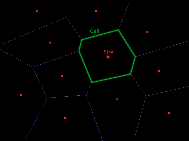
A voronoi diagram is a way of dividing up a space into a set of regions (which we call cells) given a set of input points (which we call sites), such that each cell contains exactly 1 site, and the points inside the cell are exactly those whose nearest site is the one inside that cell.

Voronoi diagrams have an extraordinarily wide range of applications. They can be used to create textures for water, generate geometry for rocky ground, efficiently calculate a point’s nearest neighbour or for guiding the movement of AI agents. All these useful applications got me excited to try some of them out myself, but this posed one rather glaring problem: How does one actually go about generating a voronoi diagram?

If you have a relatively small number of sites, then you can simply enumerate every point in your space and compute which site is closest. This works if you only care about which site each point in space belongs to and you have finitely many discrete points, for example if you just need to determine the colour for every pixel in an image.

On the other hand if you have a very large number of input points, or you care about where the boundaries between cells is then another approach is called for. There are a few ways of computing the voronoi diagram for a set of input points but the one we’ll look at today is called Fortune’s Algorithm.

In my quest to write my own implementation of Fortune’s algorithm I struggled to find many good explanations of it. There are many implementations¹ but not very many explanations. The best that I found was this one by Ivan Kutskir, though it left many questions unanswered for me. I hope to leave fewer questions unanswered for you, dear reader (and for future me)!

Fortune’s algorithm: An overview

Fortune’s algorithm takes a sweep-line approach. We consider each site in order and “grow” the cells around each site as we sweep. Once a cell has been completely surrounded by other cells, it obviously cannot grow any further. This means that we only need to keep track of those cells near to the sweep line that are still growing. We will refer to this collection of growing cells as the “beachline”.

The growing cells are represented as arcs (specifically parabolas) that grow around their site as the sweepline moves. In theory we could sweep in any direction but to keep the mathematics simple and more familiar (in terms of dealing with parabolas), our sweep line will be horizontal and will move from top to bottom.

Here is a simple example of the algorithm at work (move your mouse to see the algorithm work as the sweepline moves):

You may have noticed that most of the structural change to the beachline happens at the same time as one of two other events: Either the sweep line encounters a new site, or two cells grow large enough that they completely “squeeze” or cover the cell between them (or equivalently, when two edges in the beachline grow long enough that they intersect).

This is because the algorithm is indeed event-based. Rather than actually shift the sweep line along one pixel at a time, we maintain a queue of events that need to be processed, arranged in the order that they would be encountered by the sweep line. The two types of events are site events and edge-intersection events. In short, a site event is when we add an extra arc to the beachline, and an edge-intersection event is when we remove one. It is worth mentioning that what I call edge-intersection (or arc-squeeze) events are also referred to as circle events or arc-removal events.

In order to provide effective insertion and lookup procedures, the beachline is an ordered collection. Arcs (or growing cells) and the edges between them are kept ordered by the x-coordinate of where they appear in the beachline. Note that this is not the same as being ordered by the x-coordinate of a arc’s focus, since the beachline may contain multiple arc with the same focus.

In very high-level pseudocode, Fortune’s algorithm functions as follows:

Fill the event queue with site events for each input site.
While the event queue still has items in it:
    If the next event on the queue is a site event:
        Add the new site to the beachline
    Otherwise it must be an edge-intersection event:
        Remove the squeezed cell from the beachline
Cleanup any remaining intermediate state

Details of how to handle both events are explained below, but first:

Some mathematical background

I mentioned above that the algorithm represents growing cells as parabolas. In school most people are taught that a parabola is defined by the equation \(y = ax^2 + bx + c\). However there is another definition: Take a point (which we will call the focus) and a straight line (which we will call the directrix). Now if we were to mark all of the points on the plane for which the distance to the focus is the same as the distance to the closest point on the directrix, the resulting set of points would make a parabola.

For our purposes the directrix will always be a horizontal line, and will always be below the focus.

One issue with this definition of a parabola is that it is not necessarily obvious how one might compute the y-coordinate of the curve for some value x-value. With some manipulation (shown below) of the standard definition of the parabola and our definition of the focus and directrix, we can show that for a directrix \(y = y_d\) and focus \((x_f, y_f)\), we get the formula \(y = \frac{1}{2(y_f - y_d)}(x - x_f)^2 + \frac{y_f + y_d}{2}\).

The useful part of this definition is that it gives us a handle on the distances between things. Let us consider for a moment two curves, defined by two different points (\(f_1\) and \(f_2\)) but the same directrix, which intersect at some point \(p\). Since the curves share both \(p\) and the directrix, so their distance from \(p\) to the directrix is obviously the same. However by definition this means that the distance from \(p\) to \(f_1\) is the same as the distance from \(p\) to \(f_2\). Now if \(f_1\) and \(f_2\) are two sites in a voronoi diagram, then all points on one side of \(p\) are closer to \(f_1\) than they are to \(f_2\) (and should therefore be in the cell around \(f_1\)) and all those on the other side are closer to \(f_2\) (and should be in the cell around \(f_2\)).

Since this is true for all points \(p\) at which the two curves intersect, we can find the boundary between the two cells by moving the directrix around and drawing a line consisting of the intersection points. This is the mathematical reasoning behind Fortune’s algorithm. Although the algorithm doesn’t quite function mechanically in quite the way explained here, this is the reason why the output is a valid Voronoi diagram.

One thing I should mention though, is that I have yet to show why this intersection will always be a straight line.

Handling site events

The first type of event we need to handle is the one for when the sweep line encounters a new site. In this case, step one is finding out which existing arc our new point falls under. Conceptually we are going to split that arc into two pieces, with the arc for our new site between them.

Note that at the point where a new site is encountered, the directrix lies exactly on the new site. This means that the parabola defined by that focus and directrix is effectively a straight line extending directly upwards. This is convenient because it gives us just a single x-coordinate (namely that of the new site) to search for in our beachline. The beachline is ordered, so we can do a binary search. It is important when testing our new x-coordinate to see which branch to follow while searching, that we compare it against the intersection point of two other curves rather than the focus of one.

The cells created by our new arc (which we’ll call \(a_n\)) and the arc that the search found (\(a_f\)) will clearly be adjacent in the resulting voronoi diagram, so there needs to be an edge between them. Now while Fortune’s algorithm is running, we actually track two different types of edges: Edges that are still growing (which correspond to those that fall inside an arc on the beachline) and edges that are complete. Complete edges are what you probably think of geometrically as “edges”: each one is a straight line between to points. We will mention complete edges again later, but for now we’re only interested in edges that are incomplete and still “growing”. Some implementations refer to complete edges simply as “edges” and incomplete/growing edges as “half edges”.

A growing edge is actually more like a ray. It has a starting point and a direction and conceptually it extends out in its direction until it intersects with an arc (namely the arc that created it). We will create two edges every time a site is added to the beachline. Both new edges share the same starting point: the intersection of the new arc and that found by the search. Their directions are exactly opposite though. They are the two vectors perpendicular to the line between the focuses, one extending “to the left” and one extending “to the right”. Let’s call them \(e_l\) and \(e_r\) respectively.

Lastly we need to create to new arcs \(a_{fl}\) and \(a_{fr}\), the left- and right- splits of \(a_f\). These are essentially just two copies of \(a_f\), differing only in their place in the beachline.

We’ve created all our new beachline items, we need to actually update the beachline. So we remove \(a_f\) from the beachline and in its place, insert the sequence \(a_{fl}, e_l, a_n, e_r, a_{fr}\).

One final step before we’re finished handling this event, is to check if any new edge-intersection events need to be added to our event queue. Conceptually having two edges intersect is equivalent to having an arc on the beachline squeezed down to nothing. We only added two new edges (\(e_l\) and \(e_r\)) and they’re extending outwards in opposite directions, so there’s no way that they alone can squeeze \(a_n\). So all we do is check \(a_{fl}\) and \(a_{fr}\).

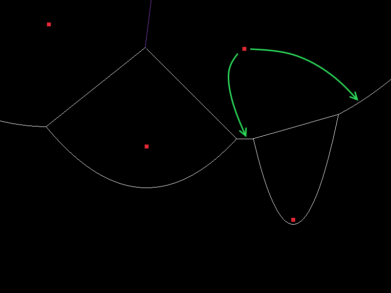
Checking for new edge-intersection events

Given a particular arc (call it \(a\)), we want to find out if we need to add an event where it gets squeezed. To do this we first find the edges to the immediate left and right of \(a\), call them \(e_l\) and \(e_r\). If either of those edges do not exist (consider that \(a\) is the left-most arc on the beachline), then we don’t need a new event. If those edges do not intersect at all (remember that they are not infinite lines, they have a “direction”) then we also don’t need a new event.

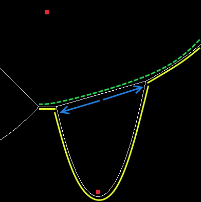
When we do need to add a new event, we need to know the y-coordinate of the sweep line, at the time of the event. To get a conceptual understanding of how we calculate that, consider that each edge is necessarily the boundary between two arcs. An edge-intersection event is the intersection of two (necessarily adjacent-on-the-beachline) edges, which gives us three arcs (the edges being adjacent means that the inner arc is the same for both edges). Since edges extend out exactly to the arc that contains them (and no further), our two edges intersecting means that all 3 of our arcs intersect at exactly this point as well. Now by the mathematical definition of our arcs, that means that all 3 focuses are the exact same distance from the intersection point.

This is why these are sometimes referred to as “circle events”: At the point of intersection we have created a circle whose centre is the intersection point and that has the focus of all three intersecting arcs on its circumference.

We still need a y-coordinate for the sweep line though, but this is simple. By definition of our arcs, the distance from the focus of the arc to the intersection point is the same as the distance from the intersection point to the directrix that forms the arc (IE our sweep line). The shortest line between the directrix and the intersection point is just a vertical line. The new edge-intersection event’s y-coordinate is therefore just the y-coordinate of the intersection point, minus the distance between the focus of any of the three involved arcs and the intersection point.

Handling edge-intersection events

When handling site events, we removed a single item from the beachline and added a sequence. Now for edge-intersection events we will remove a sequence and add a single item.

As mentioned above, two edges intersecting corresponds to the squeezing of an arc into nothingness. We clearly won’t need that arc (call it \(a_o\)) to be on the beachline anymore but we also don’t need the intersecting edges (call the left and right ones \(e_l\) and \(e_r\) respectively). So the sequence we remove from the beachline is \(e_l, a_o, e_r\). We aren’t quite finished with those edges though. I mentioned “complete edges” earlier and this is where they come in.

These two edges have intersected with each other, they’re definitely not going to grow any further which means that they now have an endpoint. So all we do is we output two “complete” edges, both with one endpoint at the intersection point for this event and with the other endpoint at the starting point of one of the removed edges.

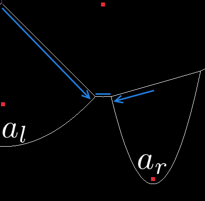
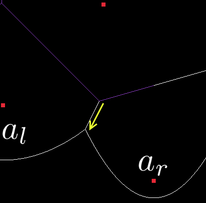
So what is it that we’re going to add to the beachline then? Well we had some edges intersect and they’re gone now, but those edges were tracking the growth of two arcs. Those arcs are still around and now they need an edge between them. So lets find the arcs to the immediate left and right of \(a_o\) on the beachline (call them \(a_l\) and \(a_r\) respectively).

The new edge needs to be perpendicular to the line between \(a_l\) and \(a_r\), and it needs to extend downwards (we only need one edges this time, not two). Simply add it to the beachline between \(a_l\) and \(a_r\). Finally, we test both \(a_l\) and \(a_r\) for new edge-intersection events, in the same way that we did above for site events.

Final steps

Once the event queue is empty, our voronoi diagram is pretty much done and we just have to tie up some loose ends. In particular we need to convert any leftover edges on the beachline into “complete” edges. The easiest way to do this is just to extend all the remaining edges out for some large amount of distance and then stop them there. If you have a pre-defined region of space that you’re working in (e.g the size of the map for a game, the edges of the image etc) then you can just extend the edges until they intersect with that.

That’s it! Your shiny new voronoi diagram is complete and you can bask in its space-partitioning glory.

Further work

So now you know something about how Fortune’s algorithm works, but that is by no means the only thing worth knowing. One (rather large) hole is that Fortune’s algorithm only works in 2D. If you’d like to have an object break apart procedural (maybe you’re smashing a large stone or piece of wood with a hammer and you want it to break up in a realistic fashion without hours and hours of artist work) then you’ll need to investigate other algorithms that work in higher dimensions.

Another thing I should probably mention is that the Delaunay Triangulation, which is the dual of the voronoi diagram. This means that its sort of the “opposite” in that you can get from one to the other very easily: The delaunay triangulation is what you get if you place edges connecting adjacent sites in the voronoi diagram (rather than placing edges between them). Delaunay triangulations are very useful in graphics (particularly for generating geometry) because they minimize the creation of “sliver” triangles which are very narrow (and therefore wasteful to render because they might only be a single pixel wide).

I hope this has proven to be a reasonably clear and intuitive explanation but feel free to let me know in the comments if there was something you didn’t understand (or if I got anything wrong). For those interested in some of the finer details or writing their own implementation, part 2 has some extra implementation detail, along with a discussion of the edge-cases that I struggled with.