Generating integers uniformly distributed over an range

You may have seen that there was recently a submission to the Swift language’s standard library with an interesting title: “An optimal algorithm for bounded random integers” by Stephen Canon. I found the idea intriguing and this post is a summary of my little expedition into the world of bounded pseudorandom integer generation.

Some background

Let us assume that we have a way to generate uniformly-distributed random bits. How we do this is its own field of research, the details and nuance of which are well beyond the scope both of this article and my own understanding. We will use a PCG generator to get random bits in this article because its one that comes to mind for me as Generally Pretty Good™.

So we have some random bits (\(N\) of them, let’s say). This is great if we want a random integer anywhere in the range \([0,2^N-1]\) but usually that is not the case. Usually we want a random number within some range that is not a power of 2. Maybe we’re shuffling a list and need a value no larger than the length of the list. Or maybe we’re playing Dungeons and Dragons and need to roll a d20 to get a value in the range \([1,20]\). In this article we will consider a situation where we want to produce a 4-bit number less than the upper-bound that we will call \(b\).

The most naive approach to turning our random byte into a random decimal digit would be to take the remainder modulo the (exclusive) upper-bound of our range. rand()%b would certainly give us a value within the desired range, but if we did this many times we would find that the results are not uniformly distributed. Consider \(b = 6\): There are three values in \([0,15]\) (the output range of our rand() function) that map to 0: 0, 6 and 12. There are also three values that map to 1, 2, and 3. However there are only two values which map to 4 (4 and 10) and the same is true of 5. So if we generated many random numbers we would find that the values 0, 1, 2 and 3 appear more frequently than 4 or 5. In addition to being biased, this method also involves doing a division by a value that is not a power of 2, which is very slow in comparison to other arithmetic operations on modern CPUs.

Producing bounded random integers quickly while still avoiding this bias is exactly the problem that we are here to investigate.

What did we do in the past?

Our problem is that the modulus takes different quantities of input values to each output value on the entire \([0,2^N-1]\) range. To visualise this lets imagine counting to \(2^N-1\) in batches of \(6\):

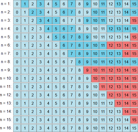
Notice how we have a bit left over at the end. We can’t fit another batch of 6 in after 11 and the remaining 4 values are the source of bias in our results. In fact just to give you a better idea, let’s take a look at this visualisation for all possible n-bit upper-bounds:

The simplest and most common strategy for solving this problem is (in a sense) to ignore it. This is the approach historically taken by the random number generators in Java and OpenBSD’s libc. If we generate a number and it falls into that part of the range which is left over when trying to “fill it” with batches of our upper bound (the red section of the figure above), then we just discard that value and generate a new one. We continue doing this until we find a value that is not within that problematic range and take the modulus with respect to our upper bound. This way we know that every possible output value is equally likely, because each one is the modulus of an equal number of random values which are themselves uniformly distributed.

def bounded_rand_javabsd(upper_bound):
    random_value = rand() # outputs a random & uniformly-distributed 4-bit unsigned value
    rand_max = 16
    max_valid_value = rand_max - (rand_max % upper_bound) - 1
    while random_value > max_valid_value:
        random_value = rand()
    return random_value % upper_bound

The only difference between the Java and OpenBSD algorithms is which side they start filling the random range from. The Java approach has us “fill from the bottom” (starting at \(0\)) and discarding values left over on the high end, which is exactly what we did in the diagram above. However, we could just as easily take the OpenBSD approach and “fill from the top” (starting at \(2^L-1\)), discarding values which are left over on the low end like so:

While we know that this approach produces uniformly-random values in the desired output range, it has the downside that it always involves at least one division by a value that is not a power of 2. We can do better.

What do we do at the moment?

The current state-of-the-art is Daniel Lemire’s “nearly divisionless” algorithm as presented in this paper (and this blog post which contains some timings). Lemire’s approach sneakily takes advantage of the fact that while the we most often get away with numbers that fit into 32 bits, pretty much all modern CPUs support 64-bit arithmetic and many languages (and some CPUs) can do 128-bit arithmetic. It still uses rejection to avoid problematic values from our random generator, but it uses the extra bits to avoid expensive divisions in many cases.

Suppose we took our (4-bit) random number and multiplied it by the size of our output range (\(6\), another 4-bit number). We now have an 8-bit number, whose value could only be a multiple of 6 in the range \([0, 6 \cdot (2^4-1)]\). If we were to divide that 16-bit number by \(2^N\) then we’d get a value in our desired range \([0,5]\). In doing so we’d be “grouping” the 16-bit range into contiguous chunks which each divide down to the same output: \([0, 1 \cdot 2^L - 1]\) divides down to 0, \([1 \cdot 2^L, 2 \cdot 2^L - 1]\) divides down to 1, etc.

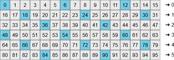
So we have a way of reducing our random value into the desired range, but we had that already in the naive solution. What’s different this time around? It would appear that all we’ve done is rearrange our bias (now it is 2 and 5 that appear less frequently). Clearly we still need to reject problematic values to make each output value uniformly likely but notice that so far we have not needed to do any divisions by a value that is not a power of two. It’ll also enable further optimisation later on.

But first, we still need to reject some values to get uniformly-likely output. In the picture above we’d like each row to have the same number of highlighted values. Those values are \(b\) distance apart and so really we’re back to our earlier problem of wanting to reject some portion of a range of 16 values so that we can batch it up evenly into groups of 6. What if we just used the same solution and reject the first \(2^N~mod~b\) of them?

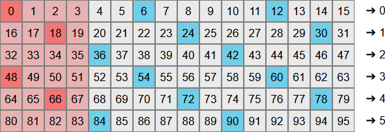
This is justified in a little more detail in Lemire’s paper but you can clearly see that each row now has exactly 2 highlighted values meaning that after dividing, our output values will all be equally likely. I’ve highlighted rejected values that are multiples of 6 in a darker shade of red and you can see we’re rejecting exactly 4 values - the same number we rejected in our earlier example using the Java/OpenBSD approach. This lends further confidence that we’re on the right track.

Once again we are now in a position where we can generate uniformly distributed values in any given range - albeit in what seems like a rather roundabout fashion. Let’s take a step back and look at some pseudocode:

def bounded_rand_slowlemire(upper_bound):
    result = rand() * upper_bound # result is an 8-bit value
    min_valid_value = 16 % upper_bound # slow division!
    while (result % 16) < min_value_value:
        result = rand() * upper_bound
    return result / 16

This almost starts out with a slow division, but here is Lemire’s crucial realisation: \((2^N~mod~b) < b\) for all \(N > 0\). Now maybe that sounds silly but hear me out: We already have \(b\). We don’t need to compute it. We can just check against it as-is. This means we can “early-out” in any case where our multiplied value lies somewhere off to the right on the diagram above. This would avoid doing any expensive division, like so:

def bounded_rand_lemire(upper_bound):
    result = rand() * upper_bound # result is an 8-bit value
    if (result % 16) < upper_bound:
        min_valid_value = 16 % upper_bound # slow division!
        while (result % 16) < min_value_value:
            result = rand() * upper_bound
    return result / 16

This is Lemire’s algorithm as presented in his paper. We still do the slow division, but only in some cases (which is why it’s only nearly divisionless). I should note though, that “some cases” doesn’t quite convey how rare such cases are. In our working example of \(N=4\) and \(b = 6\) we have a 37.5% chance of failing our early-out check and doing a slow division. That seems like quite a lot. But usually we use a few more than 4 bits to store our numbers. Usually we have at least 32 and in that case our diagram above is much, much wider. With \(N=32\) and \(b = 6\) we only have about a 0.00000014% chance. Somewhat unlikely.

This high probability to get away without doing needing any slow divisions also provides significant performance improvements over earlier approaches, as detailed both by Lemire himself in the paper and by Melissa O’Neill (the inventor of the PCG family of generators).

What is being proposed for us to do in future?

Lemire’s algorithm is good because it seldom needs to divide. But wouldn’t it be neat if we never needed to divide? Even better what if we could never divide and never reject values? That could give significant wins both in average runtime and in the variance on the runtime (which is potentially important for cryptographic applications).

Up until now every number we’ve dealt with has been an integer, both conceptually and in the sense that we ask the CPU to do integer arithmetic with them. One could (rightly) argue that Lemire’s approach treats the n-bit random integer as a fixed point value in the range \([0,1)\) but its not necessary for the approach to be easily explained.

So let us consider a different situation and forget about actual 2021-era computers for a second. Say I had a magical machine that could output a real number in the range \([0,1)\) and whose output is uniformly distributed in the sense that if I partition \([0,1)\) into any number of equally-large buckets and generate many numbers, each bucket would receive roughly the same quantity of random numbers. Now take the output of this machine and multiply it by the (exclusive) upper bound of our integer range and floor the result. Clearly what you get is a value that could be anywhere in our desired output range of integers. To see that those integers are uniformly distributed, recall that we can split \([0,1)\) into any number of buckets and get uniform output across those buckets. So split it into \(n\) buckets where \(n\) is our exclusive integer upper-bound. Each bucket is equally likely and each bucket corresponds exactly to one of the integers we could output.

Sadly we don’t have such a magical machine though. So how do we produce uniformly distributed real numbers? Recall that the only tool we have available to us is a generator that produces random bits. What we’re going to do is interpret that stream of bits as the fractional component of a fixed-point number. This is the same way normal numbers are interpreted, just with the powers shifted down: The first bit is our coefficient for \(2^{-1}\), the second is the coefficient for \(2^{-2}\) etc such that (for example) we would interpret the bits 00101 as 0.15625. So far this is nothing new though, this method has been in use for over 20 years and is known to be biased (because the range you want is probably not a power of two). The difference here is that we have a stream of random bits. A conceptually infinite stream. And the number of bits we’re going to consume from that stream is not just the size of the integer we want to output. So how many bits do we consume then?

Well if I asked you to give me an integer in the range \([0,1]\) then you’d only need 1 bit. If I asked for the range \([0,7]\) then one isn’t enough (if the first bit is a zero then it could be a 0, 1, 2 or 3). You need 3 bits for that. Now let’s say I asked for the range \([0, 5]\). With 6 possible values we have 6 buckets and bucket boundaries on every multiple of \(\frac{1}{6}\). Let’s step through it bit by bit (literally):

Let’s say the first bit is \(0\), so we know our number will be somewhere in the range \([0, 0.5)\). If the second bit is 0, that shrinks the possible range of our random real number to \([0, 0.25)\). Notice that that the bucket boundary at \(\frac{1}{6}\) is in that range. This means that our number could fall into either bucket and we need more bits to know which one it is. The next 3 bits are 1, 0 and 1, shrinking the possible range to \([0.125, 0.25)\), \([0.125, 0.1875)\) and \([0.15625, 0.1875)\) respectively. Each bit cuts the possible range in half and if at any point the possible range does not include a bucket boundary, we can stop and be sure that this was indeed our “actual” random number (in the sense that we would not have gotten a different integer end-result if we had continued adding bits).

Of course a number like \(\frac{1}{6}\) does not have a representation in this manner that is both exact and finite. However unlikely, you could potentially go on forever producing ever smaller ranges that always contain it. It’s important to note though, that the more bits we generate, the smaller our bias is. Bias in our output is the result of us producing the “wrong” value from our random bits and this is only possible if by the time we stop consuming random bits, the possible range for our real number still contains a bucket boundary. Obviously the smaller the buckets the less likely this is and the more bits we have the more buckets we have. Detecting very small bias requires producing (and analysing) a very large number of values, so as long as we use enough bits to cover the largest quantity of output we expect to produce we should be fine. Mr Canon’s implementation uses 128 bits (or more if the output value is larger than 64 bits).

Implementation

Let’s get slightly closer to the real world though: How might we implement the concept above on an actual modern computer? Well let’s first consider our real number \(r\) that is represented by the infinite random bitstream, along with our upper bound \(b\). We’ll split it after the 64th bit to get \(r = r_0 + r_1\) where \(r_0\) is the first 64 bits and \(r_1 < 2^{-64}\) is the rest of our bitstream. Recall that our final result is computed as:

$$ \begin{aligned} result &= \lfloor r \cdot b \rfloor \\ \implies result &= \lfloor r_0 \cdot b \rfloor + \lfloor frac(r_0 \cdot b) + r_1 \cdot b \rfloor \end{aligned} $$

Note that \(frac(r_0 \cdot b) < 1\) by definition. If our upper bound fits into 64 bits (which it does by definition if our API takes it as a 64-bit integer) then \(r_1 \cdot b < 1 \implies frac(r_0 \cdot b) + r_1 \cdot b < 2\) meaning that after flooring, the second term of \(r\) is either 0 or 1.

If we decide (as Mr Canon did) that 128 bits is enough to effectively eliminate bias, then we can truncate \(r_1\) at 64 bits. This makes implementation on modern CPUs fairly simple. We generate 2 random 64-bit numbers which are \(r_0\) and \(r_1\). \(r_0 \cdot b\) is then just a normal 64-bit integer multiply and produces a 128-bit number. Most (if not all) modern 64-bit CPUs support addition and multiplication of 64-bit values that might produce 128-bit results, possibly by providing the low and high bits of the result separately. \(frac(r_0 \cdot b\)\) is simply the low 64-bits of that multiplication of two 64-bit values. Similarly for the addition, leaving us with something like the following pseudocode:

def bounded_rand_canon(upper_bound)
    r0 = rand()
    r1 = rand()

    r0_hi_bits, r0_lo_bits = full_width_multiply(r0, upper_bound)
    r1_hi_bits, _ = full_width_multiply(r1, upper_bound)
    sum_hi_bits, _ = full_width_add(r0_lo_bits, r1_hi_bits)

    return r0_hi_bits + sum_hi_bits

No loops! No conditionals! (Effectively) uniformly-distributed random integers in an arbitrary range! There are some downsides of this though, it requires multiplies and adds with twice the bit-width of the result (which not all hardware necessarily supports) and it always consumes two words from the generator whereas the other approaches above only consume one (at least some of the time). If your generator is slow then requiring more bits might be an issue but there are several fast generators to choose from and it is possible to avoid computing \(r_1\) in some cases where we know it will not change the result (see the Swift implementation for an example).

One final thing to note about this though, is that the avoidance of bias in this approach depends on the total number of bits consumed from the generator. If you wanted (say) a 16-bit value, you can’t drop down to 16 bits for \(r_0\) or \(r_1\). The Swift implementation just treats all bitwidths less than 64 as if it were actually 64 and then just truncates the output (which will fit into the remaining bits by definition since the result is less than the upper-bound which was given in that many bits).

Well you got this far…

I’d like to think I’ve satisfactorily explained broadly what’s going on here, but if you’re interested in more detail I encourage you to read the original proposal (it’s fairly short). Beyond that, other sources I found useful while writing this post include this post that breaks down Lemire’s nearly-divisionless algorithm and this post which compares various existing approaches (both in terms of bias and performance).